Big-O Notation Notebook

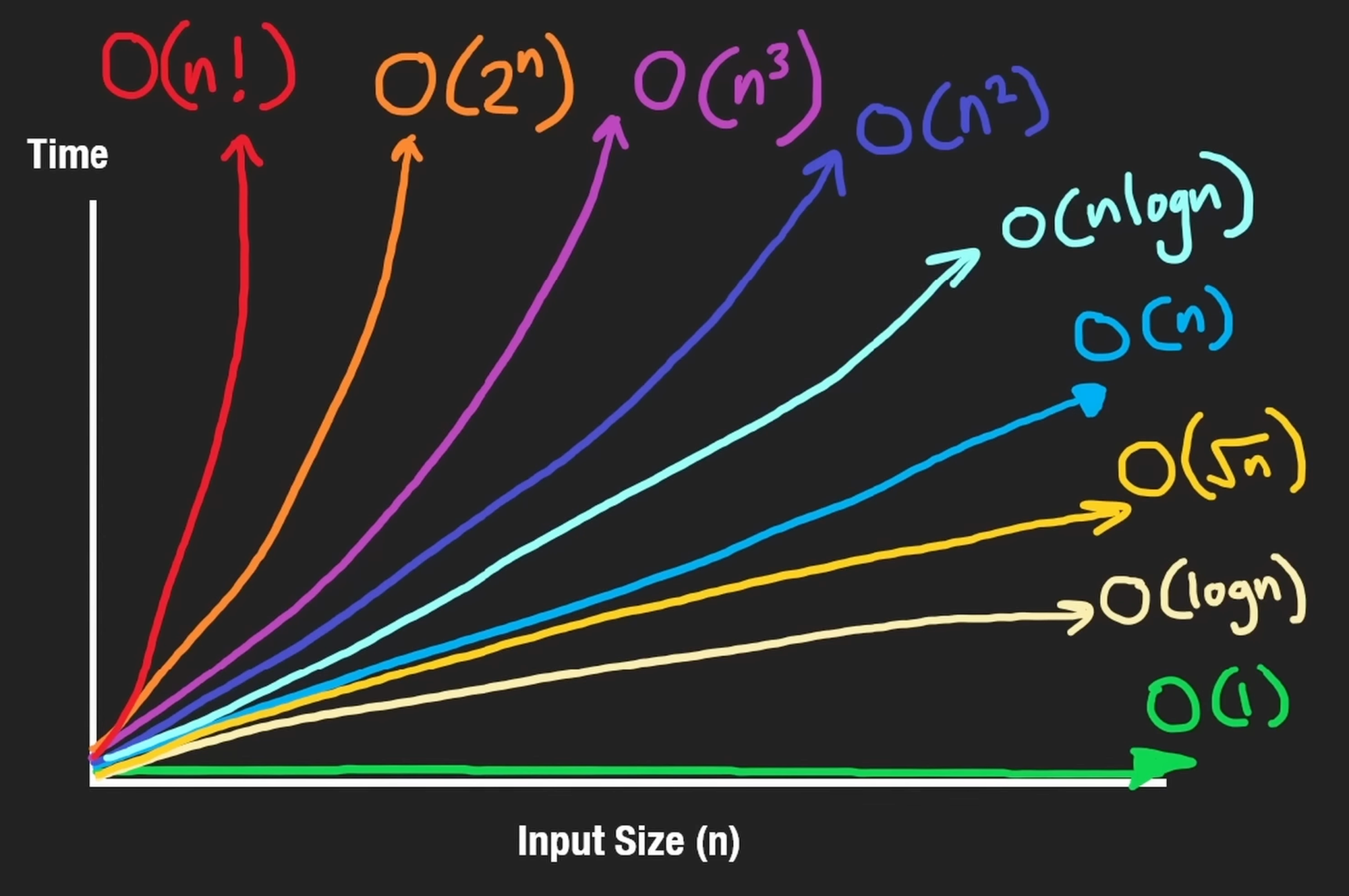
Understanding Big-O Notation

Big-O is like planning for the heaviest traffic during rush hour—it helps you understand the maximum time an algorithm might take to complete, preparing you for the worst-case scenario.

O(1): Constant Time Complexity

• Efficiency: Highest possible, as execution time remains constant regardless of input size n.
• Behavior: Performance does not change; operations complete almost instantly.

Common Examples:

• Accessing an element by index in an array.
• Adding or removing the last element in a stack (push/pop operations).
• Inserting or deleting the first element in a queue.

Coding Examples:

Array operations:

nums = [1, 2, 3]
nums.append(4)  # Append operation at the end
nums.pop()      # Pop operation at the end
print(nums[0])  # Access by index; look up

Dictionary operations:

hash_map = {'key': 10}
hash_map['new_key'] = 20      # Insert operation
print('new_key' in hash_map)  # Check existence
print(hash_map['new_key'])    # Access by key
hash_map.pop('new_key')       # Remove by key

---

O(log n): Logarithmic Complexity

• Efficiency: Highly efficient for large datasets as it reduces the problem size by half each step.
• Application: Common in algorithms that divide the problem space into smaller segments, typically seen in binary operations.

Common Examples:

• Binary Search: Quickly locates an element in a sorted array by repeatedly dividing the search interval in half.
• Binary Search Tree (BST) Operations: Efficiently find, insert, or delete nodes.
• Divide and Conquer Algorithms: Like the "Guess the Number" game, which narrows down the possible answers with each guess by halving the range.

Coding Examples:

Example of Binary Search in Python:

nums = [1, 2, 3, 4, 5]
target = 3
l, r = 0, len(nums) - 1
while l <= r:
    m = (l + r) // 2
    if nums[m] < target:
        l = m + 1
    elif nums[m] > target:
        r = m - 1
    else:
        print(f"Target found at index {m}")
        break

Example of Binary Search on a Binary Search Tree (BST):

def search_bst(root, target):
    if not root:
        return False
    if target < root.val:
        return search_bst(root.left, target)
    elif target > root.val:
        return search_bst(root.right, target)
    else:
        return True

Using a Min Heap:

import heapq
min_heap = []
heapq.heappush(min_heap, 5)  # Insert into heap
heapq.heappop(min_heap)      # Remove from heap

---

O(sqrt(n)): Square Root Complexity

• Efficiency: Uncommon but effective for certain types of problems, especially those involving factorisation or searching.

Coding Examples:

This example demonstrates how to find all factors of a number, efficiently using O(sqrt(n)) complexity by iterating only up to the square root of the number.

Finding all factors of n:

import math
n = 12
factors = set()
for i in range(1, int(math.sqrt(n)) + 1):
    if n % i == 0:
        factors.add(i)
        factors.add(n // i)
# Output the factors
print(factors)

This approach significantly reduces the number of iterations needed to find all factors of n by using a set, making it faster than a typical O(n) solution that checks every number up to n.

---

O(n): Linear Complexity

• Efficiency: Increases linearly with the size of the input. The time complexity grows directly proportional to the input size n.
• Behavior: The worst-case runtime involves iterating through all elements, making it predictable and straightforward.

Common Examples:

• Traversing an array or linked list to process each element.
• Deleting a specific position in a linked list where traversal is required.

Coding Examples:

This section demonstrates various O(n) operations in Python, including array manipulation and heap operations.

nums = [1, 2, 3]

# Summing elements of an array
total = sum(nums)
print("Sum:", total)

# Looping through the array
for n in nums:
    print("Element:", n)

# Inserting at a specific index
nums.insert(1, 100)
print("After Insert:", nums)

# Removing an element
nums.remove(100)
print("After Remove:", nums)

# Checking for element existence
print("Is 100 present?", 100 in nums)

Converting array into a heap:

import heapq
heapq.heapify(nums)
print("Heapified array:", nums)

As well as nested loops example (e.g., sliding window technique) - complexity depends on the operations inside the loop.

These examples highlight how O(n) complexity appears in typical data manipulation tasks and some algorithms where operations scale linearly with the input size.

---

O(n log n): Linearithmic Complexity

• Efficiency: Extremely effective for operations that combine linear traversal with logarithmic processes, often seen in sorting algorithms.
• Characteristics: This complexity is typical where you combine a linear process with a step that divides the problem set (logarithmically).

Common Examples:

• Merge Sort: Efficiently combines smaller sorted arrays into larger ones.
• Heap Sort: Builds a heap and then sorts by removing the largest or smallest element repeatedly.
• Quick Sort: Selects a pivot and partitions the array around it, sorting the partitions recursively.
• Certain Divide and Conquer Algorithms: Optimises O(n^2) algorithms by breaking the problem into smaller parts and solving them individually.

Coding Examples:

Here we demonstrate how heap sort and merge sort operate, reflecting O(n log n) complexity.

HeapSort example in Python:

import heapq
nums = [5, 3, 1, 4, 2]

# Building the heap from the list, O(n)
heapq.heapify(nums)
sorted_nums = []

# Removing the smallest element until the heap is empty, O(log n) each
while nums:
    sorted_nums.append(heapq.heappop(nums))

print("HeapSort result:", sorted_nums)

MergeSort example (using Python's built-in sorting which is typically Timsort):

nums = [5, 3, 1, 4, 2]
sorted_nums = sorted(nums)  # Utilizes a variation of merge sort with O(n log n) complexity
print("MergeSort result:", sorted_nums)

These examples underscore how O(n log n) operations are pivotal in efficient data processing, particularly in sorting and optimising complex algorithms.

---

O(n^2): Quadratic Complexity

• Efficiency: Common in algorithms that involve pairs of elements or nested iterations, leading to performance that scales as the square of the input size.
• Characteristics: Often observed in simpler or brute-force sorting algorithms and when dealing with two-dimensional data structures.

Common Examples:

• Bubble Sort: Repeatedly steps through the list, compares adjacent elements and swaps them if they are in the wrong order.
• Insertion Sort: Builds the final sorted array one item at a time by inserting elements at their correct position.
• Selection Sort: Repeatedly selects the smallest (or largest) element from the unsorted portion and moves it to the end of the sorted portion.
• Traversing a 2D Array: Iterates over each row and column of a matrix.

Coding Examples:

These examples demonstrate typical scenarios where O(n^2) complexity occurs, including iterating through a 2D array and implementing a basic sorting algorithm.

Traverse a square grid in Python:

nums = [[1, 2, 3], [4, 5, 6], [7, 8, 9]]
for i in range(len(nums)):
    for j in range(len(nums[i])):
        print(nums[i][j], end=' ')
    print()

Get every pair of elements in an array:

nums = [1, 2, 3]
for i in range(len(nums)):
    for j in range(i + 1, len(nums)):
        print(f'Pair: ({nums[i]}, {nums[j]})')

Example of Insertion Sort:

def insertion_sort(nums):
    for i in range(1, len(nums)):
        key = nums[i]
        j = i - 1
        while j >= 0 and key < nums[j]:
            nums[j + 1] = nums[j]
            j -= 1
        nums[j + 1] = key

nums = [3, 2, 1]
insertion_sort(nums)
print("Sorted array:", nums)

These snippets underline the impact of quadratic complexity, especially evident in data processing and sorting operations where each element must interact with others in a nested manner.

---

O(n*m): Multiplicative Complexity

• Efficiency: Encountered in situations where the performance depends on the product of two different dimensions, such as in rectangular grids or operations involving two different datasets.
• Characteristics: Similar to O(n^2) in scenarios where both dimensions can vary independently.

Common Examples:

• Cross-product Operations: Generating all possible pairs from two different lists or arrays.
• Traversing a Rectangular Grid: Iterating through each cell of a grid that does not necessarily have equal dimensions (e.g., a 2x3 grid).

Coding Examples:

The following snippets illustrate how O(n*m) complexity manifests, by showing operations on arrays of different lengths and a rectangular grid traversal.

Get every pair of elements from two different arrays:

nums1, nums2 = [1, 2, 3], [4, 5]
for i in range(len(nums1)):
    for j in range(len(nums2)):
        print(f'Pair: ({nums1[i]}, {nums2[j]})')

Traverse a rectangular grid:

nums = [[1, 2, 3], [4, 5, 6]]
for i in range(len(nums)):
    for j in range(len(nums[i])):
        print(nums[i][j], end=' ')
    print()  # New line after each row

These examples highlight the computational considerations when dealing with operations that require accessing elements across two dimensions or datasets, each influencing the total number of operations performed.

---

O(n^3): Cubic Complexity

• Efficiency: Generally inefficient due to the high runtime, especially as the size of n increases. Often impractical for large datasets.
• Characteristics: Typically appears in algorithms that involve three nested loops, affecting performance significantly as each layer adds another dimension of iteration.

Common Examples:

• Triple Nested Loops: Used to generate all possible triplets from an array, which is common in certain mathematical or brute-force solutions.

Coding Example:

This example illustrates a simple cubic complexity scenario where all unique triplets from an array are printed. Such operations are computationally intensive and usually avoided in performance-critical applications.

Print all unique triplets in an array:

nums = [1, 2, 3]
for i in range(len(nums)):
    for j in range(i + 1, len(nums)):
        for k in range(j + 1, len(nums)):
            print(f'Triplet: ({nums[i]}, {nums[j]}, {nums[k]})')

This code efficiently demonstrates an O(n^3) complexity by iterating through three nested loops to produce every combination of three elements without repetition. The example is straightforward, highlighting the nature of cubic complexity in a clear and concise manner.

---

O(2^n) / O(c^n): Exponential Complexity

• Efficiency: Highly inefficient for large values of n due to the exponential growth in the number of operations.
• Characteristics: Often associated with recursive functions where the number of recursive calls doubles or increases by a constant multiplier at each step.

O(2^n):

• Use Case: Commonly appears in recursive algorithms that explore all possible combinations or paths, such as in computing the Fibonacci sequence or solving decision problems.
• Example: Computing the Fibonacci sequence recursively where each call generates two further calls.

Coding Example for O(2^n):

Fibonacci sequence using recursion, which doubles the calls at each step:

def fibonacci(n):
    if n <= 1:
        return n
    return fibonacci(n - 1) + fibonacci(n - 2)

# Testing the function
print(fibonacci(5))  # Output: 5 (0, 1, 1, 2, 3, 5)

O(c^n):

• Explanation: This complexity arises when the recursive function expands by more than two branches per call, typically influenced by an additional variable or parameter c, which can sometimes be dependent on n.

Coding Example for O(c^n):

General exponential recursion where c branches out depending on the input size:

def exponential_recursion(i, nums, c):
    if i >= len(nums):
        return 0
    total = 0
    # The loop creates multiple branches per recursion, depending on c
    for j in range(1, c + 1):
        if i + j < len(nums):
            total += exponential_recursion(i + j, nums, c)
    return total

# Example usage with c branches
nums = [1, 2, 3, 4, 5]
c = 3
print(exponential_recursion(0, nums, c))  # Output depends on specific conditions and `nums` length

Both examples illustrate the complexity and potential inefficiencies of exponential growth in recursive algorithms, particularly when the problem size or parameters allow recursive calls to multiply rapidly. These complexities are typically avoided in practical applications unless optimisations or memoisation techniques are applied to reduce the impact of redundancy in recursive calls.

---

O(n!): Factorial Complexity

• Efficiency: Extremely slow and typically impractical for large n due to the exponential increase in the number of operations required.
• Characteristics: Factorial complexity occurs in scenarios where you need to generate all possible permutations of a dataset, which grows factorially with the number of elements.

Common Examples:

• Travelling Salesman Problem (TSP): Solved via brute-force search by evaluating every possible route to determine the shortest possible path.
• Generating Permutations: Producing all possible orderings of a set without any restrictions.
• Laplace Expansion: Used to compute the determinant of a matrix, where each expansion adds factorial growth in complexity.
• Set Partitions: Enumerating all distinct ways to partition a set into non-empty subsets.

These examples involve extensive computations as the input size increases, making them highly inefficient for larger datasets. Due to the nature of factorial growth, such complexities are often theoretical or restricted to very constrained or small-scale problems in practical applications.

Big-O Notation Cheat Sheet

Complexity	Description
O(1)	Constant - The fastest and most efficient complexity, where operations complete in the same time regardless of the input size.
O(log n)	Logarithmic - Efficiency scales with the logarithm of the input size, typical in binary search.
O(n)	Linear - Runtime grows directly in proportion to the input size.
O(n log n)	Linearithmic - Combines linear and logarithmic complexities; common in efficient sorting algorithms like mergesort.
O(n^2)	Quadratic - Often results from nested loops; each element is processed multiple times.
O(n^3)	Cubic - Similar to quadratic, but with three nested loops; less common due to high inefficiency for large data sets.
O(2^n)	Exponential - Doubling with each additional element; common in recursive algorithms solving the subset problems.
O(n!)	Factorial - The slowest and least efficient; associated with algorithms that generate all permutations of a dataset.
O(n^n)	Exponential - Extreme cases where the complexity grows exponentially with the number of elements raised to their own power.

---

Notes for Myself

• Case such as n + nlogn, we don't need to say the first n because in Big-O notation we only care about the larger term if they are the same variable. so we can just say: nlogn.
• BUT, case like m + nlogn, we have to mention the m in m + nlogn because m is a different variable.

---

References:

• https://neetcode.io/courses/lessons/big-o-notation
• https://stackoverflow.com/questions/1592649/examples-of-algorithms-which-has-o1-on-log-n-and-olog-n-complexities